Regression Models and Spiders in Virtual Reality

After watching the movie Inception many years ago, I thought about what it would take to create a computerized “multiplayer dreaming” system. With the recent news about brain-machine interfaces, my interest in this field has been piqued once again in the form of this proposed research experiment involving dreaming spiders.

Objective

The goal of this experiment is to approximate patterns between the brain patterns of spiders and corresponding leg motions. Eventually, this research might be used to not just transmit data from an organism’s brain to a computer, but the other way around.

With this data, ideally we would be able to create a neural network which can take an input of brain wave patterns and output where the spider’s legs would be.

The spider

The experiment starts with the choice of species. To ensure consistency in different labs, the spiders should all be as similar as possible. In order for us to image its brain waves, we’ll need to genetically modify the organisms, so the species should have well-documented genetic data.

For practicality in the lab, the spiders should be easy to breed and not too aggressive or cannibalistic.

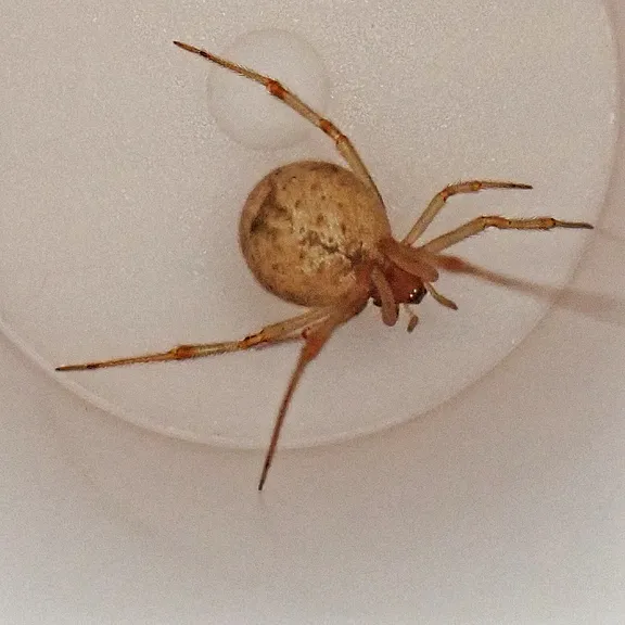
This is Parasteatoda tepidariorum. It’s known as the common house spider, and was chosen for this because of its long history of being used in studies.¹ In 2017, Schwager et al. sequenced the genome of P. tepidariorum, meaning that we have the knowledge of how the base pairs relate to each other and how each section influences the function of the organism.² This allows our genetic tooling for genome editing to work effectively.

In the lab, we’d set up housing for the spiders, feeding schedules, and temperature and humidity controls. The goal at this stage is to collect roughly a few hundred individuals and record the attributes of each. This allows us to have records which later allow for analysis of how those variables affect our model.

Genetic Engineering

A spider’s locomotion relies on patterns that spread throughout its “brain”. To be specific, a spider has a large mass of neurons in its cephalothorax called a ganglion. In orb-web spiders, research observed that the section of nerves above the esophagus (called the supraesophageal ganglion) connects to the spider’s eyes and manages vision, while the lower mass (called the subesophageal ganglion) controls the abdomen and appendages.³

To achieve a model which can accurately predict leg movements from neural activity, a few electrodes measuring electric pulses at tiny points wouldn’t be sufficient. A comprehensive image which shows the entire pattern of how the nerves in the ganglion light up is needed.

Fortunately, there has been research done in this area. GCaMP is a genetically encoded calcium indicator which visualizes neural activity in real time. When genetically engineered into a genome, neurons emit green light during activation. It’s super reactive and we can see visual feedback in neurons within 2 milliseconds.⁴

In our spider population, we’d design a way to deliver the genetic material. Most likely, gene editing technology like CRISPR-Cas9 would be used to insert GCaMP until we get a successful embryo. Genotype spiderlings to tell which ones have the gene, and then repeat until we find two with GCaMP in germline cells, which develop into eggs or sperm. Once we collect enough individuals with the gene present in the germline, breeding them will yield more GCaMP-positive spiders for later use.

Setup

The spider’s movements have to be measured precisely, and any external influences could contaminate our data. Firstly, we’d have to put the spider into an isolated container. The outside air currents shouldn’t be perceived by the spider. To solve the problem of the spider feeling vibrations on the floor of the container, we have to suspend it from the top. I imagined the harness going around the cephalothorax and between the legs (the harness must be fine enough to not interfere with legs). The string suspending the spider must also be elastic so as to not transfer the vibrations. Spring constants and damper specifications can be calculated from lab-gathered data.

As shown in Fig. 2, with the elastic harness, resonant vibrations from HVAC systems, footsteps, and traffic won’t affect the spider or our data. Now, with our spider fixed in place, we can begin the neural imaging.

Imaging

To image the ganglion, we’ll use two-photon microscopy. The conventional method used to be one-photon imaging, which worked like this:

1. You shine a single photon into the mass of nerves.
2. The photon excites GCaMP and it emits green light.
3. Your camera collects the green light and creates an image.

This method was extremely limited. Excitation happened all along the light path, not just the 3d area you wanted to image. If you were imaging under tissue, your photons could scatter and your emission would have noise. The specimen would also get damaged unnecessarily, since emission light is harmful to live organisms.

Two photon microscopy improved on these issues significantly:

1. You shine a laser emitter that fires photons with half the energy
2. Due to optics, these photons get progressively denser near the focus and spread out everywhere else
3. Since each photon has only half the energy, GCaMP is only activated by two photons colliding

Since emission only activates when two photons collide and this practically only happens at the focal point of the laser, we image only the small area we want. This reduces our noise and phototoxicity issue.⁵ Now, this only targets a small area surrounding the focal point of the laser, but we need to observe macroscopic patterns to make a useful regression model.

First, to focus on an area closer or further from our laser, the previously used method was moving the objective lens. As shown in Fig. 3, the convex lens causes the parallel light rays from the laser to converge at a distance from the lens, marked by the purple dots. Moving the lens moves this convergence point, or “focus”.

The problem with this approach is that the lens we have to move is heavy and has inertia. When we try to move it rapidly, it starts resisting our motion, overshooting and vibrating. This ruins our signal and limits us to roughly 10-100 images per second.

Chakraborty et al. in September of 2020 found a way around this problem. To understand their solution, we’ll first have to understand the galvanometric mirror. The system centers around the goal of moving a mirror as fast and as precisely as possible.

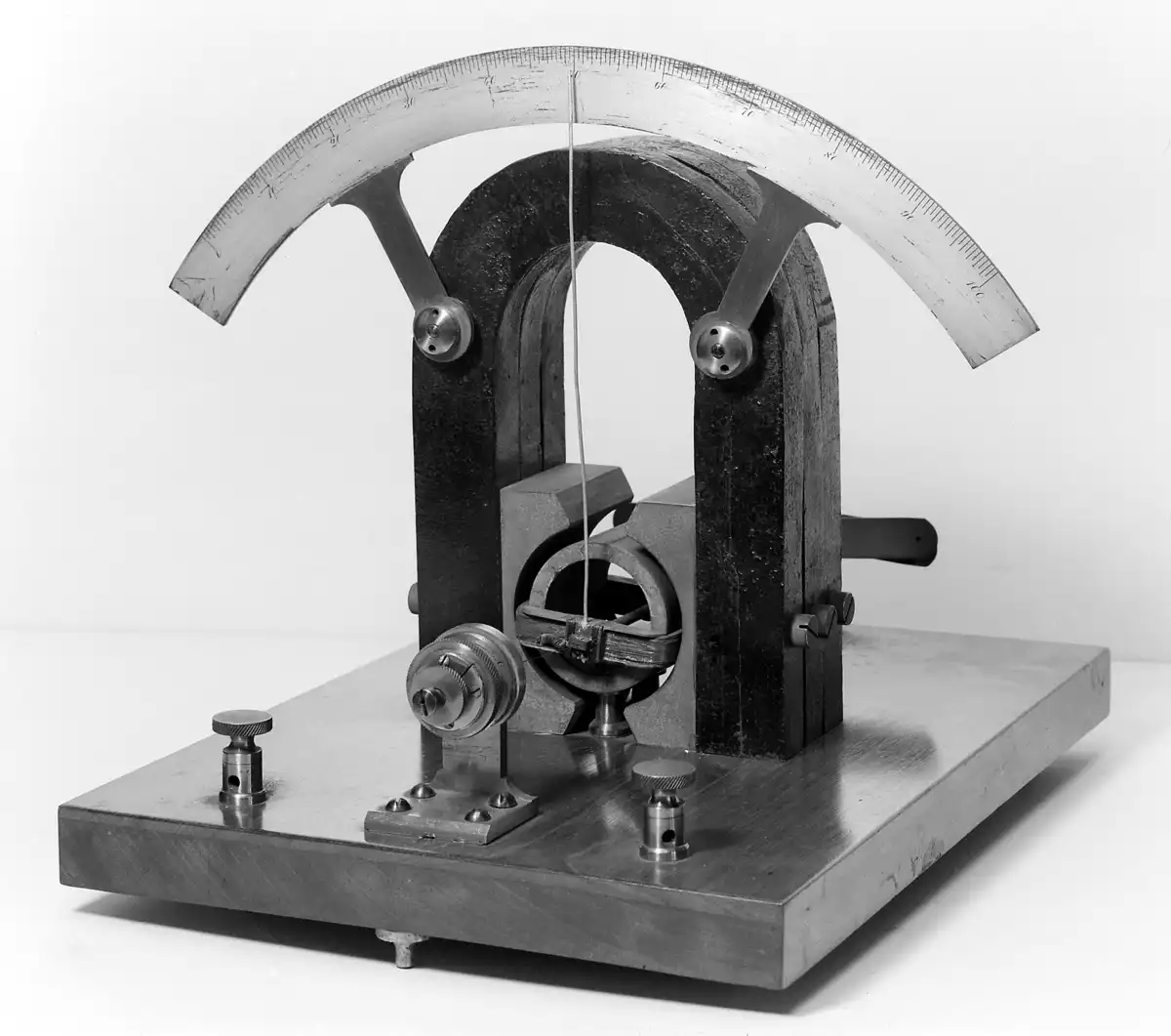
The early galvanometer’s purpose was to measure tiny currents. Fig. 4 shows an 1882 d’Arsonval moving coil galvanometer, which used a stationary magnet and a current-carrying coil. When current passed through the coil, Lorentz force made it rotate and react to changes in current.

Very quickly, it was noticed that the coil moved only a tiny angle. That meant attaching a mirror to the rotating segment would allow us to move the mirror very precisely and through electricity. With a computerized system, the current passing through the coil could be orchestrated with the lasers, which enables scanning in X and Y directions.

There are two ways to use galvo mirrors: as a servo and as a vibrator. When used as a servo, you send an electrical signal and a feedback loop works to adjust the coil to your desired angle. This makes it manipulatable and gives a wide variety of scan patterns, but due to mechanical inertia, you are limited in frequency of scans. When used as a vibrator, it’s mounted on a spring vibrating at resonant frequency and the coil simply provides enough energy to keep it going.⁶

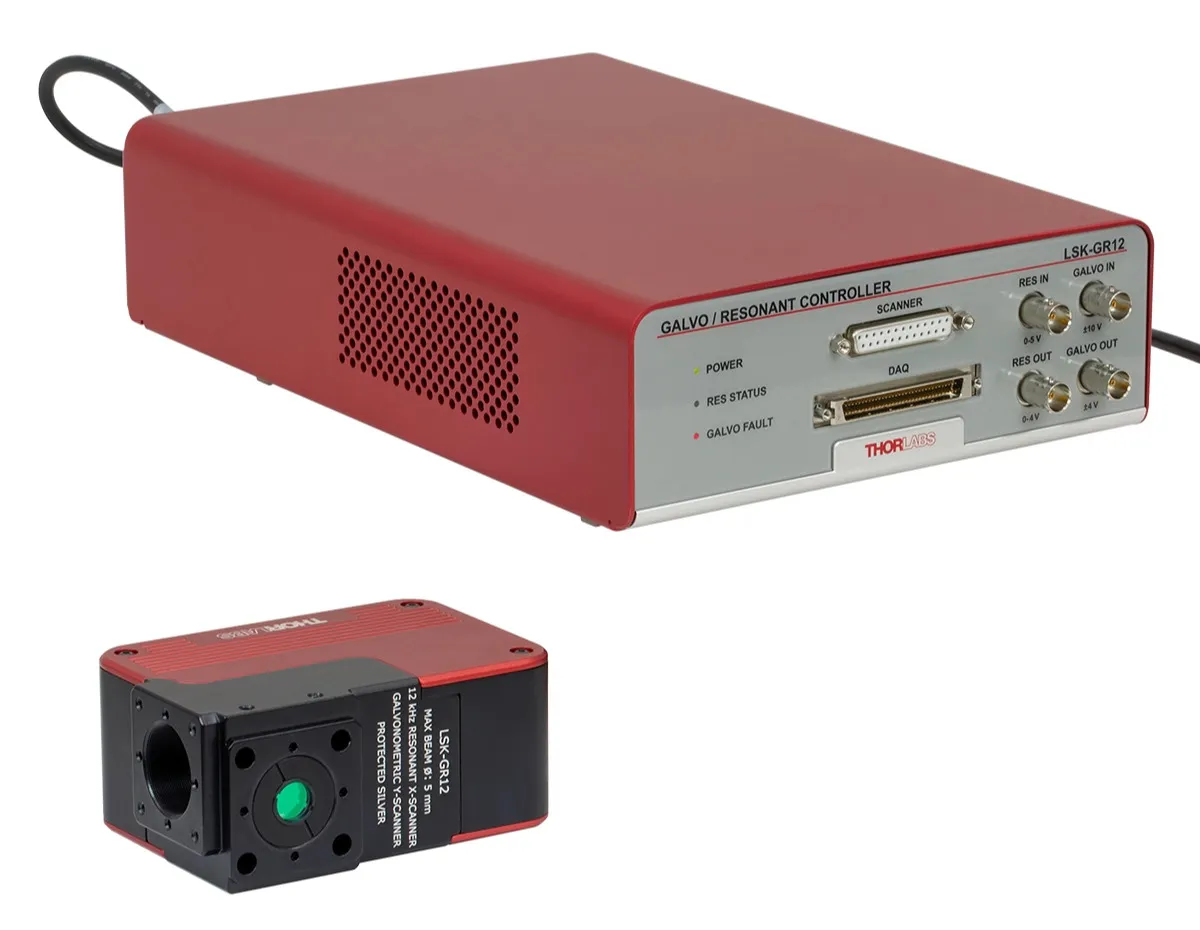
The main breakthrough that the vibrator uses is using the galvanometer as a supporter. The mirror itself isn’t being driven by torque from an electric feedback loop, but instead the natural resonant frequency of a very stiff spring. The galvanometer just releases energy at the right times so that energy loss from friction and heat don’t stop it entirely. Fig. 5 shows what a modern version of this looks like, specifically the Thorlabs LSK-GR08.

Chakraborty et al. utilized the fact that a mirror has much less mass than a lens. A moving objective lens has to manipulate light rays through it and is made of glass, making it heavy. A mirror only has to reflect light waves, so it can move way faster. Their solution was to remove the moving objective lens altogether and go for a remote focusing arm. The remote focusing arm is a third resonant galvo (vibrator) that is placed at a tilted angle relative to the laser. As the spring oscillates, the remote focusing mirror tilts the focus of the photons along the depth axis while the other two resonant galvos sweep across the X and Y axes. This allowed them to image brain tissue in three dimensions at 12 kHz.⁷

With our spider in the harness, we’d cut a window in its dorsal cuticle. This is the thin layer of chitin covering its dorsal surface and is commonly known as a carapace. This window helps us get a clear view at the ganglion, since photons that go through chitin spread around and mess with our image. To prevent the ganglion from drying out and killing the spider, we need Ringer’s solution.

Ringer’s solution is water mixed with salts that match osmotic balance to prevent cell collapse. This is probably a bit of a tangent, but osmosis itself is a pretty interesting thing to understand.

Essentially, there are water particles on both sides of the cell membrane. On the inside of the cell membrane are ions, and on the outside of the cell is pure distilled water with no ions at all. Water molecules are in constant random motion, bouncing around and occasionally hitting the membrane. The membrane has tiny channels called aquaporins which only water molecules can rush through. In equilibrium, equal numbers of water particles pass in and out of the membrane.

The catch? Ion solvation shells. Inside the cell, ions like sodium and calcium attract water molecules into hydration shells. As shown in Fig. 6, ions attract water molecules into a shell-like structure, which becomes too big to enter an aquaporin. This makes more inbound water molecules than outbound water molecules. As more water molecules enter the membrane, it starts stretching, but the internal pressure isn’t enough to meaningfully increase outbound water traffic since it expands instead of resisting. Much before internal pressure would allow equalization of inflow and outflow, the membrane explodes from excessive internal water pressure. This is called lysis. However, much before lysis occurs, messing with the ions in our specimen would cause irreversible damage to its neurons and it would be brain dead well before lysis occurs.

Now, finishing the imaging setup. We create a solution that emulates the ions in its hemolmyph to keep the ganglion hydrated and drop it through the carapace window. Calibrate the two photo microscope to take a high frequency three dimensional stream of neural activation data in its ganglion, and we should have a decently accurate heatmap.

Tracking

We need a source of truth to base our model on. Remember, the goal of this project is to be able to feed our neural network the stream of ganglion activation and have it output the state of its legs. To do that, we need to know the relative 3D positions of each leg joint and tip.

This requires a bespoke motion capture setup, and I’ve envisioned it to account for the size of the spider. Usually, motion capture is done by fixing reflective IR balls to landmarks on the actor’s body and using epipolar geometry to track where they are located in 3D space. However, the average female P. tepidariorum weighs about 40 milligrams⁸ and there is no way we could attach enough reflective balls to measure its movement without interfering with its legs.

The idea is to paint each joint of its leg with an IR-reflective paint. Each landmark needs at least two cameras shooting it at the same time, so we would have 5-8 calibrated high-shutter-speed cameras placed everywhere around it (excess due to occlusions from legs curling). There would definitely be challenges with tracking any organism at this scale. The legs are incredibly thin and each reflective IR blob would be sub-millimeter in radius. Confusions in identifying two landmarks that overlap would likely be common.

Fig. 7 shows the landmarks in one spider leg. 4 per leg with 8 legs means 32 points that need to be individually tracked and identified.

If you are actually following this experiment, this might be a big challenge. I’m just writing this as a theoretical, so the implementation details of how to track a spider’s limbs in 3D space aren’t going to be available to me. However, you can refer to 2021 research by Boehm et al. for inspiration.⁹ Perhaps it would be possible to train a CNN on manually labeled harnessed spider images from a bunch of angles and that would help with landmark identification.

Anyways, real-time high-res image processing won’t be necessary. You can take synchronized recorded tracks of neural activity from two-photon and leg landmark data and then compare afterwards. This should be feasible on any robust scientific machine with a dedicated GPU.

Finally, it’s time for the last segment of the research project: machine learning.

Regression

I’m no ML expert, which is probably why the majority of this article focuses on the biology aspects of this article. But I roughly know the inputs and outputs required, so this section can offer a high-level overview.

With our Galvo-Resonant imaging, we can get a 3D array of neuron activations (X, Y, and depth), but we need a way to serialize it for input in the model. For this, consider splitting the ganglion into voxels and calculating the intensity of each voxel at each point in time. Voxels should be small enough to capture details from the original image.

The output should be an IK target for each leg at any $t + \Delta t$, since there’s a small delay between neural activity and its reflection in the leg. Inverse kinematics since a spider leg is constrained in certain ways and less landmarks to predict is better for accuracy.

First thing in the pipeline is normalizing and preprocessing data. With our voxels, apply denoising filters and normalize all the fluorescence signals. Also, since GCaMP is really fast to reach fluorescence after neuron activation but is significantly slower to drop back down, the signal might be ghosted (an image showing remnants of past signals). To solve this, we could either train the model with this data since the newest signals would be brightest, or we could make a deconvolution model.

The deconvolution model would take in our voxel data and output it so that it reflects the actual present electrical signals, filtering out the ghosts of previous ones. I suggest using glass microelectrodes. These can reach tip diameters of half a micrometer or less, which is really good for the scale of a P. tepidariorum brain.¹⁰ The electrode would give real-time electric signals of tiny points in the ganglion. Using that information, you could train a neural network to remove the ghosting from voxel data.

As for leg landmarks, convert them into joint angles so the network can meaningfully learn to output inverse kinematics. We can use radians for the angle data or normalize to something else. Doesn’t matter too much.

Neural delay should be fairly easy to account for. Signals in the ganglion precede the leg movements by some amount of time, and we can measure empirically with glass electrodes and high speed cameras. TTL (transistor-transistor-logic) can pulse on the scale of nanoseconds, so we can use that as the shared clock. We can input this as data for each individual specimen if the delay has too high of a spread.

For modeling the relationship, use temporal regression. The model needs memory of previous neural and leg states, since a spider’s walk depends on the previous states of its legs and ganglion. We can use GRU (gated recurrent unit) for this purpose. Input sequences are short windows of the ganglion. Output should be leg IK targets. We can set constraints for biologically possible positions that the leg can be in, which reduces the output space by a lot, since a spider’s legs mostly curl inwards and outwards.

Finally, we can keep iterating on this with loss functions and repeating with a wide variety of spiders until our model gets to a high degree of accuracy. If the model’s predicted trajectories line up with the tracked landmarks, it’s a success.

Future work

With the temporal regression weights, we can finally predict how a spider moves based on a 3D voxel scan of its brain. You might be wondering what exactly the purpose of this is.

Obviously, this is work that I’d want to later see done with humans, but the technology is far away. The human brain is much more complex, but this research is more of a proof-of-concept.

My idea with this was a “spider virtual reality”. It would involve us harnessing a bunch of these spiders into their own chambers, suspending them in midair. Then we could calibrate them and “drop” them inside a virtual world. I chose P. tepidariorum partly because of the genetic documentation, but also because it mainly relies on vibrations for perception.

It would be remarkable if we could surround the spider with vibrating surfaces, or even put a platform under its legs to give it the feedback loop of walking. Then, for our convenience, we might visualize it interacting with its environment with a rigged 3D model. Imagine making a spider believe it was in its web and that it felt the vibration of prey when in reality, it was suspended in one of our labs, and the prey was really a vibration motor. That would certainly be something.

Thank you for reading this article. That is all. Until next time, I am out.